Determination of cutoff values for biomarkers in clinical studies

Sook Young Woo; Seonwoo Kim

doi:10.23838/pfm.2019.00135

Abstract

In clinical and epidemiological studies, biomarkers are associated with disease diagnosis and prognosis. Using biomarkers to classify subjects into groups, such as high-risk or low-risk, may help with the application of the most appropriate care or procedure within each group. In the case of a continuous biomarker, a cutoff value to define the groups should be determined. A widespread and straightforward method is to select a cutoff value that minimizes the P-value when comparing the outcomes between the two groups. However, a problem that arises with this procedure is that of multiple testing, which leads to an increase in false positive error rate, and thus the significance of the obtained cutoff value tends to be overestimated. In this article, we introduce several methods to correct the P-value for determining the statistical significance of an optimal cutoff value for a quantitatively measured biomarker with applications to clinical data.

Keywords: Biomarkers; Corrected p-value; Cutoff; False positive error

INTRODUCTION

In clinical and epidemiological studies, biomarkers are associated with disease diagnosis and prognosis, the two major determining factors for managing a patient’s care. For this purpose, biomarkers can be used to divide patients into two groups, such as high-risk or low-risk groups, which have statistical and clinical advantages. A continuous variable may have clinical significance concerning the outcome, but its effects may be non-linear or non-monotonic [1]. Patient classification into two groups based on the presence of a biomarker may help to apply different care or procedures to each group. For example, it may be helpful to divide lung cancer patients into two groups based on tumor size and to apply radiotherapy or pneumonectomy to each group, to provide the most effective treatment. However, the method for choosing the actual cutoff is not straightforward and many possible approaches are available for such classification. A cutoff can be selected without using data, where a priori biological reasoning, a clinician’s experience, or published results are considered. Although, the choice of a cutoff based on the clinician’s experience may depend on his or her criteria, cutoffs may vary due to difference of subjects across previous studies [2-4]. Statistical methods based on data are also applicable for estimating new cutoff values.

There are two statistical approaches for determining a cutoff value: biomarker-oriented and outcome-oriented. The biomarker-oriented approach splits a continuous marker about some percentile or the mean of biomarker values. In contrast, the outcome-oriented approach selects the biomarker cutoff that takes into account the association between outcome and biomarker. The outcome-oriented approach is expected to provide a better cutoff value than the biomarker-oriented approach [5]. Even though the biomarker-oriented approach is a simple exploratory method, it may fail to select a cutoff related to outcome. The cutoff estimated by the outcome-oriented approach can be applied to predicting patient prognosis. This article describes several methods of statistical inference used to estimate and test cutoff values, with a focus on the outcome-oriented approach.

METHODS

Minimum P-value approach

A widespread, straightforward method is to select a cutoff value that corresponds to the most significant difference in the prognosis of an outcome between the two groups and one that provides the minimum P-value among all potential cutoffs. Cutoff values are determined from the entire range (minimum, maximum) for a biomarker or from a selected range, which excludes clinically non-relevant cutoff values. For example, in a data set with a size (n=10), a binary outcome (Y=0, 1), and a continuous biomarker (X), the data sets are examined to determine what cutoff value best separates the two groups. For each potential cutoff, c, the investigator draws a 2×2 table and then selects a cutoff value that maximizes the chi-square statistic, while equivalently minimizing the P-value (P_min) (Table 1). However, with such a procedure, the problem of multiple testing arises. This means that the significance of the chosen cutoff value tends to be overestimated [6-10]. Adjustment approaches have been developed to resolve the increase in false positive error rate.

Adjustment methods to correct P-values

Bonferroni method

To protect from the increase of false positive error rate, a new P-value is obtained by multiplying the minimum P-value by the number of tests performed.

P_bon=P_min×the number of tests performed

In the Table 1, the chi-square test is conducted for each c and the corrected P-value for the cutoff corresponding to P_min, P_bon, equals P_min×9. This method is relatively easy for calculating the corrected P-value and can be applied to any type of outcome. However, the method is conservative, and with more candidate cutoff values it becomes more difficult to reach statistical significance.

Miller and Siegmund method

The Miller and Siegmund method [11] selects the interval of a continuous biomarker, X, (X(ε), X(1-ε); 0<ε<0.5) which is symmetric in the tail areas. For example, with ε=0.1, the range of candidate cutoffs of X is selected as (10th percentile, 90th percentile). Among the potential cutoff values within the interval (X(ε), X(1-ε); 0<ε<0.5), the asymptotic distribution of the maximum chi-square statistic regarding binary outcome is derived and the formula for the P-value corresponding to the cutoff with the maximum chi-square statistic using this distribution is as follows:

P(1)=ϕ(z)z-1zlog1-ε2ε2+4ϕ(z)z

where z is the 1-pmin2 percentile in the standard normal distribution and ϕ (z) is the value of the probability density function of the standard normal distribution at z. For example, in the case of P_min=0.05, z is the 97.5th percentile in the standard normal distribution, 1.96, and ϕ (1.96) is 0.975. This method is less conservative than the Bonferroni method because multiplication of the minimum P-value by the number of tests performed is not necessary, but this method can only apply to binary outcome and is inappropriate for small data sets. Additionally, the results of this method depend on the selection of the value of ε.

Lausen and Schumacher method 1

This approach [12] generalizes the Miller and Siegmund method so it can be extended to asymmetric ranges (X (ε1), X (ε2); 0<ε1<ε2<1) of candidate cutoff values for a biomarker. If the investigator excludes the lower 5% and the upper 10% of the biomarker data, the cutoff value is searched within the interval (5th percentile, 90th percentile). The P-value corresponding to the cutoff with P_min is computed using the following formula:

P(2)=ϕ(z)z-1zlogε21-ε11-ε2ε1+4ϕ(z)z

This method has the advantage that it can be applied to data with ordinal outcome, continuous outcome and time to event outcome as well as binary outcome, but it has the same disadvantage as the Miller and Siegmund method concerning small data sets.

Lausen and Schumacher method 2

Lausen et al. [13] developed a formula for the P-value using an improved Bonferroni’s inequality and asymptotic method [14,15] when the number of candidate cutoff values is not very high (50 to 100). This method also considered the correlation between the test statistics for adjacent cutoff values. The equation is as follows:

P(3)=21-ϕz+∑i=1k-1Dli,li+1

where l_i is the number of observations which is less than or equal to i^th candidate cutoff value (i=1,…,k-1). The value of the function of D is calculated with the following formula:

D(i,j)=1πexp-z22tij-z24-1tij36, with tij=1-i(N-j)(N-i)j

This formula can be also applied to binary outcome, ordinal outcome, continuous outcome and time to event outcome. We recommend to use the smaller of P-values of P⁽²⁾and P⁽³⁾ [16].

Contal and O’Quigley method

This method provides a P-value that is derived from an asymptotic distribution of an adjusted statistic for the log-rank test to compare survival curves [17]. The equation is as follows:

P(4)=2∑i=1∞-1j+1exp-2j2q2, where q=1sk-1maxLk

where L_k is the log-rank statistic computed at the k^th candidate cutoff value, and s is calculated with 1(k-1)∑j=1kaj2 (where, a_j is the score for j^th event and equals 1-∑i=1j(1k-i+1)). The power for this method is comparable to the power of the Lausen and Schumacher methods. The Contal and O’Quigley method has the advantage of having a higher power and lower bias for data when there is a high proportion of censoring and the data set is not small.

Woo et al. method

Competing risk is an event that either hinders the observation of the event of interest or modifies the chance that this event occurs. For example, after a bone marrow transplantation, when studying leukemia relapse, non-relapse death can be considered as a competing risk. With these types of data, a popular method to compare survival curves is Gray’s test [18]. Woo et al. [19] developed a P-value derived from the asymptotic distribution of the modified statistic (q’) for Gray’s test and the equation is shown below.

P(5) = 2∑i=1∞-1j+1 exp-2j2q'2, where q'=1s'k-1maxGk

G_k is the Gray’s statistic calculated at the k^th cutoff value and s is calculated with 1k-1∑j=1k a'j2. a′ is defined as the Gray’s statistic type. This method provides small bias and high power for data without censoring, but the results from this method are not optimal for data with a high proportion of censoring.

Table 2 summarizes the types of outcomes and the various adjustment approaches for correcting P-values to prevent an increase in false positive error rates due to the multiple testing problem that occurs during the process of inference for biomarker cutoff value determination.

Software packages for the Miller and Siegmund method, the Lausen and Schumacher methods 1 and 2, and the Hothorn and Lausen method are available in the R package (R Foundation for Statistical Computing, Vienna, Austria) “maxstat”. Also, package “survMisc” in the R can be used for the Contal and O’Quigley method. Woo et al. method was implemented in a SAS macro (SAS Institute Inc., Cary, NC, USA), and code will be made available upon request.

APPLICATIONS

Leukocyte elastase and coronary artery disease

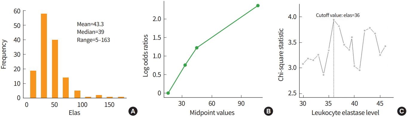
The data from 141 subjects were collected to investigate the clinical usefulness of leukocyte elastase in the diagnosis of coronary artery disease (CAD) [20]. The mean, median, and range of leukocyte elastase were 43.3, 39.0, and 5 to 163, respectively. To explore the possibility that a cutoff exists, the log-odds ratio for each quantile of leukocyte elastase data was examined. Fig. 1 graphically presented that a cutoff around the median value 39 may divide the subjects into two groups. Since the outcome, CAD, is a type of binary data, four methods to select a cutoff using a corrected P-value can be applied, and the results from each method are displayed in Table 3. The leukocyte elastase cutoff is estimated to be 36 from all methods. The minimum P-value approach provided a significant P-value of 0.0014, which does not correct for the false positive error rate increase. The corrected P-value from the Bonferroni method is the largest as expected, and the P-values resulting from the other methods, P⁽¹⁾, P⁽²⁾, and P⁽³⁾ were all significant. The results demonstrate that we can divide the subjects into two groups regarding CAD using a significant cutoff of 36 for leukocyte elastase.

Mean gene expression level and death in diffuse large B-cell lymphoma patients

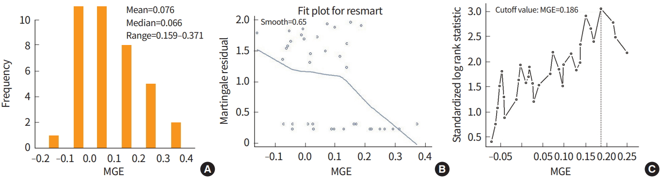
In data from 38 lymphoma patients (http://llmpp.nih.gov/lymphoma/data.shtml) [21], a cutoff value for mean gene expression (MGE) was estimated to classify the patients into low-risk or high-risk of death groups. Among 38 patients, 20 patients died and 18 patients were censored during the study period. The mean, median, and range for the MGE were 0.076, 0.066, and –0.159 to 0.371, respectively. Martingale residuals for survival model were examined to determine if there was a possible cutoff for MGE. The residual slope decreased rapidly after approximately 0.1 and the probability of death may be different between the two groups if classifying by an MGE cutoff of 0.1 (Fig. 2).

Because the outcome of this data is death, which is a time to event, we could determine an MGE cutoff for the prognosis of death in lymphoma patients using the Contal and O’Quigley method as well as the Bonferroni method, and the Lausen & Schmacher methods 1 and 2. From these methods, the estimated MGE cutoff value was the same at 0.186 and the P-values corresponding to this cutoff were all significant except for the Bonferroni method result (Table 4).

Tumor size and recurrence in lung cancer patients

The data from 758 lung cancer patients undergoing tumor removal from 1991 to 2005 were collected. The data consisted of tumor size (cm) as a biomarker for recurrence. In this data, death after surgery was treated as a competing risk event. Among 758 patients, 580 patients had recurrences, 65 patients died without a recurrence, and 113 patients were censored. The distribution of tumor size was skewed to the right, with a median, mean and range of 3.0, 3.3, and 0.0 to 19.0, respectively. A Martingale residual plot showed a non- linear pattern of association between tumor size and time to recur and demonstrated a possible cutoff for tumor size around 3.0 cm. The rightmost plot in Fig. 3 shows that the standardized Gray’s statistic is maximized at a tumor size of 2.7 cm. With this cutoff value, the P-value was <0.0001 when applying the Woo et al. method.

CONCLUSION

Biomarkers, which can be measured as continuous or categorical data types, play a role as risk factors or predictors of clinical outcomes. In clinical practice, biomarker data, which is usually a continuous measurement, is often divided into two categories based on an optimal cutoff value. This kind of categorization makes it easier to interpret the effects of a biomarker on the outcome via an odds ratio or risk ratio. It also helps clinicians by providing objective criteria in the selection of treatment options. In this article, we focused on the dichotomization of continuous biomarkers and presented several methods to resolve the problem associated with the increase in false positive error rate, which occurs during multiple testing. We summarized the methods according to the type of outcome and presented some of their applications.

Miller and Siegmund method [11] is relatively easy to use, but it is appropriate to use only for binary outcome. For ordinal, continuous outcomes in addition to binary outcomes, Lausen and Schumacher methods [12,13] can be applied. And, when the outcome of interest is time to event, Lausen and Schumacher methods [12,13] and Contal and O’Quigley method [17] can be applied where competing risk is not taken into account. Contal and O’Quigley method [17] has the advantage of having a higher power and lower bias than Lausen and Schumacher methods [12,13] when there is a high proportion of censoring in the data. Woo et al. method [19] can be used for time to event outcome considering competing risk event and this method is powerful under no censoring. When there is a high proportion of censoring in outcome with competing risk event, an empirical P-value based on a lot of permuted samples is closer to the nominal level than the approximate test.

There are possibilities associated with the loss of information from the data, including a decrease in the power for detecting statistical significance and the biased estimation in the process of categorizing a continuous biomarker. Therefore, the cutoff value should be estimated after fully examining the feasibility of categorization using both clinical and data-driven factors [22,23].

CONFLICTS OF INTEREST

No potential conflict of interest relevant to this article was reported.

Notes

AUTHOR CONTRIBUTIONS

Conception or design: SYW, SK. Acquisition, analysis, or interpretation of data: SYW, SK. Drafting the work or revising: SYW, SK. Final approval of the manuscript: SK.

ACKNOWLEDGEMENTS

This work was supported by grant of National Research Foundation of Korea (No. NTX1170701), Republic of Korea

Fig. 1.

Histogram of leukocyte elastase (A), values showing the log odds ratio against the mid-point values for each quartile of elastase (B), and a plot of a standardized two-sample statistic against elastase values with the vertical line representing an elastase cutoff value of 36 (C).

Fig. 2.

Histogram of mean gene expressions (MGE) (A), martingale residuals against MGE and their smoothed curve (B), and plot of the standardized log rank statistics against the MGE values with the vertical line representing an MGE cutoff value of 0.186 (C).

Fig. 3.

Box plot of tumor size (A), martingale residuals against tumor sizes and their smoothed curve (B), and a plot of the standardized Gray’s statistic against tumor sizes with the vertical line indicating a 2.7 cm tumor (C).

Table 1.

2×2 Table for the data set divided by a cutoff

	X≤c	X>c
Y=1	n11	n12
Y=0	n21	n22

n11, n12, n21, n22 are respective cell counts corresponding to c.

X, continuous biomarker; c, a candidate cutoff value; Y, binary outcome.

Table 2.

Approaches for optimal cutoff value determination by outcome type

Outcome type	Adjustment methods
Outcome type	Bonferroni method	Miller & Siegmund method	Lausen & Schumacher method 1	Lausen & Schumacher method 2	Contal & O’Quigley method	Woo et al. method
Continuous	V		V	V
Binary	V	V	V	V
Ordinal	V		V	V
Time to event (without CR)	V		V	V	V
Time to event (with CR)	V					V

CR, competing risk.

Table 3.

P-values corresponding to a leukocyte elastase cutoff of 36 for the diagnosis of coronary artery disease in each method

	P_min	P_bon	P^a)	P^b)	P^c)
P-value	0.0014	0.1445	0.0026	0.0012	0.0007

P_min, minimum P-value approach; P_bon, Bonferroni method.

^a) P was calculated using Miller & Siegmund method;

^b) P was calculated using Lausen & Schumacher method 1;

^c) P was calculated using Lausen & Schumacher method 2.

Table 4.

P-values corresponding to a mean gene expression cutoff of 0.186 for the risk of death in each method

	P_min	P_bon	P^a)	P^b)	P^c)
P-value	0.0263	0.9731	0.036	0.024	0.0344

P_min, minimum P-value approach; P_bon, Bonferroni method.

^a) P was calculated using the Lausen & Schumacher method 1;

^b) P was calculated using the Lausen & Schumacher method 2;

^c) P was calculated using the Contal and O’Quigley method.

REFERENCES

1. Lee JH, Park SK, Ryoo JH, Oh CM, Choi JM, McIntyre RS, et al. U-shaped relationship between depression and body mass index in the Korean adults. Eur Psychiatry 2017;45:72–80.

2. de la Rochefordiere A, Asselain B, Campana F, Scholl SM, Fenton J, Vilcoq JR, et al. Age as prognostic factor in premenopausal breast carcinoma. Lancet 1993;341:1039–43.

3. Marubini E, Mezzanotte G, Boracchi P, Veronesi U. Long term survival analysis: breast cancer and age at diagnosis. Stat Med 1990;9:737–48.

4. Ribeiro GG, Swindell R. The prognosis of breast carcinoma in women aged less than 40 years. Clin Radiol 1981;32:231–6.

5. Kuo YF. Statistical methods for determining single or multiple cutpoints of risk factors in survival data analysis [dissertation] Columbus (OH): Division of Biometrics and Epidemiology, School of Public Health, The Ohio State University; 1997.

6. Altman DG. Categorising continuous variables. Br J Cancer 1991;64:975.

7. Altman DG, Lausen B, Sauerbrei W, Schumacher M. Dangers of using “optimal” cutpoints in the evaluation of prognostic factors. J Natl Cancer Inst 1994;86:829–35.

8. Courdi A, Hery M, Chauvel P, Gioanni J, Namer M, Demard F. Prognostic value of continuous variables in breast cancer and head and neck cancer. Dependence on the cut-off level. Br J Cancer 1988;58:88–90.

9. Hilsenbeck SG, Clark GM, McGuire WL. Why do so many prognostic factors fail to pan out? Breast Cancer Res Treat 1992;22:197–206.

10. McGuire WL, Hilsenbeck S, Clark GM. Optimal mastectomy timing. J Natl Cancer Inst 1992;84:346–8.

11. Miller R, Siegmund D. Maximally selected chi-square statistics. Biometrics 1982;38:1011–6.

12. Lausen B, Schumacher M. Maximally selected rank statistics. Biometrics 1992;48:73–85.

13. Lausen B, Sauerbrei W, Schumacher M. Classification and Regression Trees (CART) used for the exploration of prognostic factors measured on different scales. In: Dirschedl P, Ostermann R, editors. Computational Statistics. Heidelberg (DE): Physica-Verlag; 1994. p. 483–96.

14. Hunter D. An upper bound for the probability of a union. J Appl Probab 1976;13:597–603.

15. Worsley KJ. An improved Bonferroni inequality and applications. Biometrika 1982;69:297–302.

16. Lausen B, Schumacher M. Evaluating the effect of optimized cutoff values in the assessment of prognostic factors. Comput Stat Data Anal 1996;21:307–26.

17. Contal C, O’Quigley J. An application of changepoint methods in studying the effect of age on survival in breast cancer. Comput Stat Data Anal 1999;30:253–70.

18. Gray RJ. A class of K-sample tests for comparing the cumulative incidence of a competing risk. Ann Stat 1988;16:1141–54.

19. Woo S, Kim S, Kim J. Determining cutoff values of prognostic factors in survival data with competing risks. Comput Stat 2016;31:369–86.

20. Amaro A, Gude F, Gonzalez-Juanatey R, Iglesias C, Fernandez-Vazquez F, Garcia-Acuna J, et al. Plasma leukocyte elastase concentration in angiographically diagnosed coronary artery disease. Eur Heart J 1995;16:615–22.

21. Alizadeh AA, Eisen MB, Davis RE, Ma C, Lossos IS, Rosenwald A, et al. Distinct types of diffuse large B-cell lymphoma identified by gene expression profiling. Nature 2000;403:503–11.

22. Altman DG. Categorizing continuous variables. In: Armitage P, Colton T, editors. Encyclopedia of biostatistics. Chichester (UK): John Wiley; 1998. p. 563–7.

23. Royston P, Sauerbrei W, Altman DG. Modeling the effects of continuous risk factors. J Clin Epidemiol 2000;53:219–21.